Will I (Re-)Discover a Pulsar?
By astro-marwil ; M. Wilhelm , Berlin , Germany
Introduction
Many members/participants/users/volunteers are asking themself and in the forums:
Do I have a chance with my small PC against these really big crunchers?
How high is my chance to take a discovery or rediscovery of a pulsar?
Is this chance really statistically distributed?
With this contribution I try to answer these questions by analyzing the list of ABPS-Rediscoveries published 11th July 2010. Futhermore we will get interesting insights by the distributions of the effective crunching capabilities of the participants.
Method
I transferred the list into the spreadsheet program of OpenOffice 3.2.1. The new list became several times very careful compared with the original one and corrected, since the transfer was done manually. In a second step the data were transferred to Excel 2010. The graphs and some evaluations were then analyzed with Origin 8.1, a scientific data evaluation and representation program.
Results
Some evaluations of the full list
Table 1: Per Catalog
How often a pulsar catalog does occur in the list
PSR Catalog | Quantity | Relative Quantity |
| | |
ATNF psrcat | 164 | 82,0% |
PALFA | 29 | 14,5% |
DMB | 7 | 3,5% |
| | |
Sum | 200 | 100,0% |
Table 2: Per Pulsar
How often a pulsars name does occur in the list
Multiple Rediscoveries | Quantity | Total | Relative Quantity | Relative Total |
| | | | |
8 | 1 | 8 | 0,86% | 4,00% |
5 | 3 | 15 | 2,59% | 7,50% |
4 | 4 | 16 | 3,45% | 8,00% |
3 | 14 | 42 | 12,07% | 21,00% |
2 | 25 | 50 | 21,55% | 25,00% |
1 | 69 | 69 | 59,48% | 34,50% |
| | | | |
Sum | 116 | 200 | 100,00% | 100,00% |
Table 3: Per User 1
How often a user ID-number does occur in the list of user 1
Rediscoveries | Quantity | Total | Relative Quantity | Relative Total |
| | | | |
20 | 1 | 20 | 0,65% | 10,00% |
10 | 1 | 10 | 0,65% | 5,00% |
7 | 1 | 7 | 0,65% | 3,50% |
4 | 1 | 4 | 0,65% | 2,00% |
3 | 2 | 6 | 1,29% | 3,00% |
2 | 4 | 8 | 2,58% | 4,00% |
1 | 145 | 145 | 93,55% | 72,50% |
| | | | | |
Sum | 155 | 200 | 100,00% | 100,00% |
Table 4: Per User 2
How often a user ID-number does occur in the list of user 2
Rediscoveries | Quantity | Total | Relative Quantity | Relative Total |
| | | | |
9 | 1 | 9 | 0,63% | 4,50% |
8 | 1 | 8 | 0,63% | 4,00% |
7 | 1 | 7 | 0,63% | 3,50% |
5 | 1 | 5 | 0,63% | 2,50% |
4 | 1 | 4 | 0,63% | 2,00% |
2 | 14 | 28 | 8,86% | 14,00% |
1 | 139 | 139 | 87,97% | 69,50% |
| | | | |
Sum | 158 | 200 | 100,00% | 100,00% |
Table 5: Per User(1+2)
How often a user ID-number does occur in the list of user 1 and user 2
Rediscoveries | Participants | Total | Relative Participants | Relative Total |
| | | | |
25 | 1 | 25 | 0,34% | 6,25% |
19 | 1 | 19 | 0,34% | 4,75% |
10 | 2 | 20 | 0,68% | 5,00% |
9 | 1 | 9 | 0,34% | 2,25% |
7 | 1 | 7 | 0,34% | 1,75% |
4 | 1 | 4 | 0,34% | 1,00% |
3 | 4 | 12 | 1,35% | 3,00% |
2 | 19 | 38 | 6,42% | 9,50% |
1 | 266 | 266 | 89,86% | 66,50% |
| | | | | |
SUM | 296 | 400 | 100,00% | 100,00% |
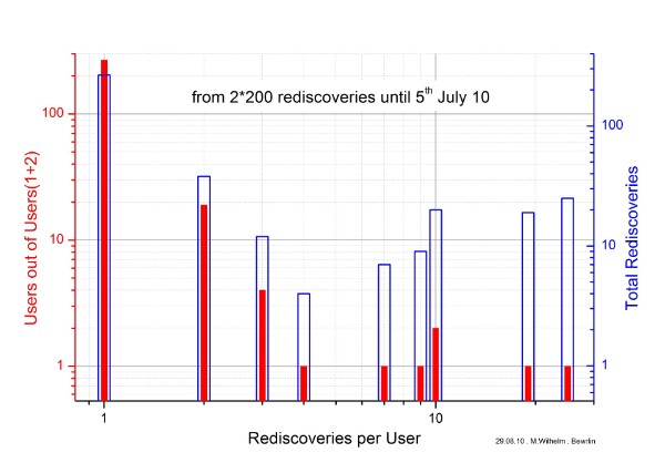
Figure 1: Number of Users as function of rediscoveries per user
From table 5 we can learn that:
90% of the ´successful´ users have a single rediscovery,
2/3 of the total rediscoveries are a single rediscovery.
This impressively shows the importance of the great community of volunteer computing!
The differences between user 1 and user 2 may be noticeable for some one. The remarkable higher rediscoveries of the top crunchers in user 1 may result from the much faster turn-around time, as Bernd Machenschalk noticed in one of his threads. (I couldn´t find this reference again.)
Some evaluations from a subset of the list
To get information about the influence of the crunching power on the number of rediscoveries per user, one requires data which are close in time related. So the following table A2 is derived from a subset from the full list of ABPS-Rediscoveries in the time interval 26th May 10 till 5th July 10 (period of announcements 27th May 10 and 11th July 10) evaluated for User 1 and User 2. This is a compromise between a high number of events and a short time interval.
The following 2 graphs show some dependency from the crunching power RAC (Recent Average Credit) and work of the ´successful´ participants TC (Total Credit).
Note: The whole list embodies 4 participants without a user ID-number. Furthermore, one ID-number is no longer listed in http://www.boincsynergy.com/ stats/ boinc-stats.php?id=xxxxx&project=eah (xxxxx=ID-number). They all got to be of country unknown and taken out of most of the following evaluations.
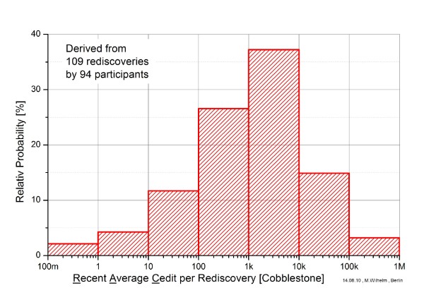
Figure 2: Distribution of the Crunching Power
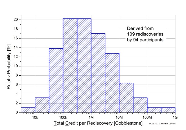
Figure 3: Distribution of the Crunching Work
The distributions show statistical behavior, but can´t be fitted nicely by any well-known distribution.
The following figures 4 to 7 are derived from all participants .
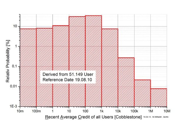
Figure 4: Distribution of the Crunching Power
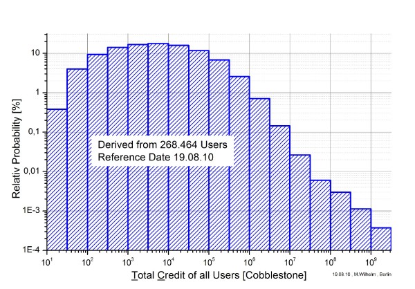
Figure 5: Distribution of the Crunching Work
It attracts attention the great different numbers of all users for RAC and TC. For RAC I did count users only with RAC≥0,01[Cobblestone]. For TC this is not so easy possible. It would need a special filter to be programmed.
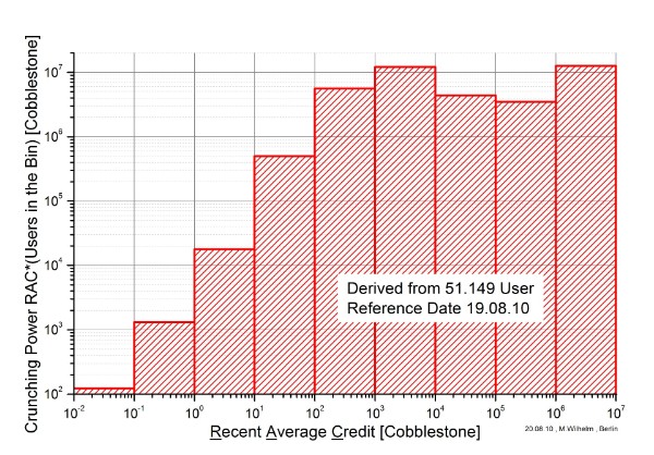
Figure 6: Crunching Power in the Bin of RAC
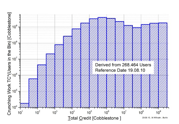
Figure 7: Crunching Work in the Bin of TC
These graphs show clearly, that the crunching power and work of the great community of volunteers can compete with the big crunchers. Nevertheless at the right side of the graphs there are not only the big crunchers as AEI eScience group and Caltech Open Science Grid but also a few volunteers who conduct big farms of PCs.
To compare the countries is not only interesting for people who are thinking in national categories, as these values of RAC and TC comprise not only the data of the lucky ´successful´ users, but from all participants in the countries. From table A2 in the appendix part c) we can learn, that the 30 nations who had rediscoveries take 87,8% of all users, 91,0% of the total RAC and 92,2% of the total TC.
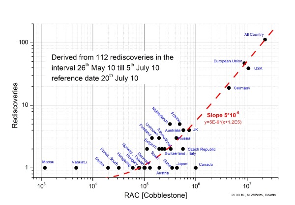
Figure 8: Rediscoveries by Countries as Function of their RAC
Discussion
It is astonishing to see the strong variation of RAC for one rediscovery by a factor of 1000. For example Canada had bad luck, whereas Netherlands with 5 rediscoveries and just 1/3 of the RAC compared to Canada had good luck. With increasing rediscoveries, the variation of RAC shrinks. This shows the role of statistics. Please keep in mind that both scales are logarithmic. So it shows relative errors. The distribution is obviously asymmetric especially at the lower rediscovery values. This can simply be explained: With increasing RAC it becomes more and more likely to get higher scores. So the really lucky crunchers with high RAC will be found at higher numbers of rediscoveries, like the above comparison Canada-Netherlands. As far as I know, these are not simple Gaussian/Normal or Poissonian distributions, as the individual members don´t have the necessary equal basis, as the vast majority of members change their activity during time (see Poisson_ distribution and appendix part a).
To estimate the proportionality between rediscoveries and RAC a manual fit was done (dotted line in figure 8). The slope of the fitting line can be estimated to be a bit lower if supposed to fit the most dense parts of the graph. But nevertheless let it be 5*10-6 [Rediscoveries / Cobblestone] within the 41 days of the observation time, that´s about 5*10-5 [Rediscoveries / (Cobblestone*year)].
For my personal data: RAC ≈ 3*103 [Cobblestone], TC ≈ 9*105 [Cobblestone], which gravitate in most foregoing graphs into the peak regions, I can calculate 5*10-5 [Rediscoveries / (Cobblestone*years)] * 3*103 [Cobblestone] = 0,15 [Rediscoveries / year].
That means I have a chance of about 2/3 to get a rediscovery or discovery within another about 7 years. This is a long journey, and not very likely to happen within the duration of the running project. By increasing the RAC by a factor of 7, which seems to be achievable also for some private persons, the necessary mean crunching time reduces to 1 year. All that assumes, that the crunching power and the density of PSRs at the observed sky area are constant throughout that time.
So this estimation is a rule of thumb: It gives an impression about the necessary remaining time and work to be done. And those participants, who don´t have the luck of a (re-)discovery are not unsuccessful, as they generate the information, there is - with the given sensitivity etc. - at this time no PSR in this region. This of course is by far the dominant case, but still of some scientific value.
Conclusions
The analysis show:
1) The majority of work is still done by volunteer computing, as 90% of the ´successful´ users have a single rediscovery and 2/3 of the total rediscoveries are a single rediscovery. The really big crunchers usually have more than one rediscovery.
2) The combined great community of volunteers can compete by RAC and TC with the really big crunchers.
3) With a rule of thumb, you can calculate your chance to take a rediscovery or discovery. The necessary factor for your RAC is about 5*10-5 [Rediscovery/(Cobblestone*year)].
4) The chance to take a rediscovery increases linearly with the activity of the participant.
5) There are strong indications for a pure statistical behavior of the system, but I believe there is no way to fit them to a well-known model. See appendix part a).
It seems to be feasible, that very similar factors as reported above will take place for the discovery of gravitational waves.
As the overall activity, in particular the relative ratio of the activity of different groups of participants – for example countries - changes very slowly, there is no need to repeat this study in close time.
Acknowledgment
At first, many thanks to my wife, as it took much, much more time than expected.
I like to say many thanks to my good old friend Dr. M. Str. in the south-west of Germany, who had a careful look on this study and made the guesses, to give it a more concise title, clearer structure and more concentrated text. I hope, I did it.
Appendix
a) Change of activity of the participants by time
All well-known statistical distributions require equal preconditions for all events within the field of observation. In our case that mean, that all participants would have to crunch with a constant RAC throughout the observation time 26th May 10 till 5th July 10. This can´t be proofed, due to lack of information, A possible approach was, to multiply the operational days by the RAC and divide this by the TC for each successful participant. This figure Change of Activity do become:
a) = 1 for a participant who did crunch all time constantly,
b) < 1 for a participant who reduced his activity,
c) > 1 for a participant who spend more time and/or a better computer.
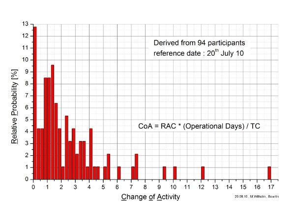
Figure A1 : Relative Occurrence of the Change of Activity
Table A1 : Change of Activity
| CoA< 0,75 | 0,75≤CoA<1,25 | CoA ≥1,25 |
RP | 21% | 17% | 62% |
Participants | 20 | 16 | 58 |
Rediscoveries | 18% | 19% | 63% |
“ | 20 | 21 | 68 |
16 participants and/or 21 rediscoveries in the middle, best suited class would be a too small statistical basis.
The data from a system that changes indefinitely its parameters can´t be fitted by a fixed law.
But anyhow one can´t fit the data, it seems to be credible, that they are statistical.
b) RAC as a valid measure of activity
The values of RAC are shown only for the valid total crunching work done and they differ for S5GC1- and ABPS- files by S5GC1/ABPS = 250/200. So it is necessary that the relative amount of valid ABPS-files of the total valid files is constant during the interval of interest. Otherwise one would have to correct for this. Figure A2 does show that we had luck of a sufficient stable relative amount of ABPS-files during our time interval of interest. Furthermore one can see that it could be possible to correct for changes of this relative amount within limited time ranges.
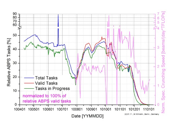
Figure A2: Relative amount of ABPS-files
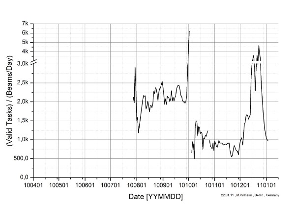
Figure A3 : Valid Tasks per Beam
c) Further Tables
Unfortunately the tables A2 to A4 are too big to be shown here. If you´r interested in that, please send an email to astro-marwil@urmawil.de, I´ll send you a pdf-version of this with the charts.
29.10.10 , Berlin , Germany
completed 25.11.10 , Berlin , Germany
corrections 30.11.10 , Berlin , Germany
Fig A2 exchanged and Fig A3 added 20.02.11 , Berlin , Germany
This study became published at 18th Nov. 2010 here.


Discover")


